Introduction to Neural Network
Abstract
I’ve been interested in Neural Networks recently and I’ve started to study about it. Here is how I understood the basics of Neural Network. (The sources I’ve referenced the most when learning was MIT OpenCourse Lecture and O’Reilly recent Machine Learning Book)
Table of Contents
- Basic Structure of Neuron
- Basic Concept of Neuron Applied for Computers Visualized
- Elaboration on Neural Network Optimization
- Applying Concepts into Python (with Tensorflow)
Basic Structure of Neuron
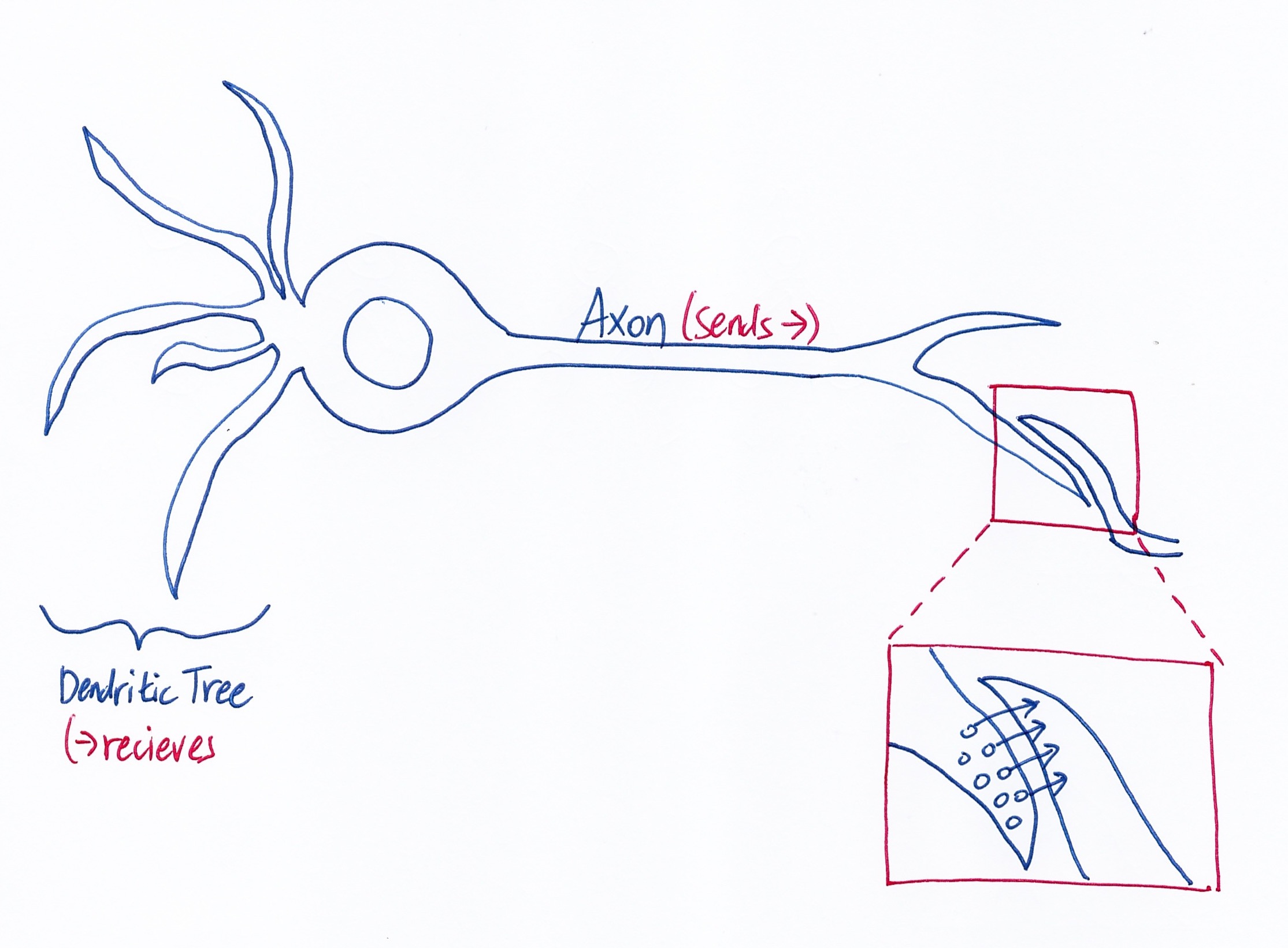
Basically, there are multiple neurons that communicate with each other by receiving information with dendritic tree and sending information with axon. As you can see in the close up part, they don’t send just 1 signals, but multiple signals. Those multiple signals either makes the other neuron stimulated or not (basically it’s either 0 or 1). However, we care about the bigger picture, so we will only care if the whole signals result to 0 or a 1 (i.e. a single neuron). Since each neuron have different weights. The ‘learning’ part is applied to these weights. We will optimize the weights so that it is closest to the actual result. Deep learning will tweak the weights according to how much it contributes to the error so that at the end, the optimization is more closer to the actual result
Basic Concept of Neuron Applied for Computers Visualized
For simplicity, I’m going to ignore about weights for this section, and just stick with 0 and 1. In the O’Reilly ML Book, it has this tree like diagram showing simple logical computations.
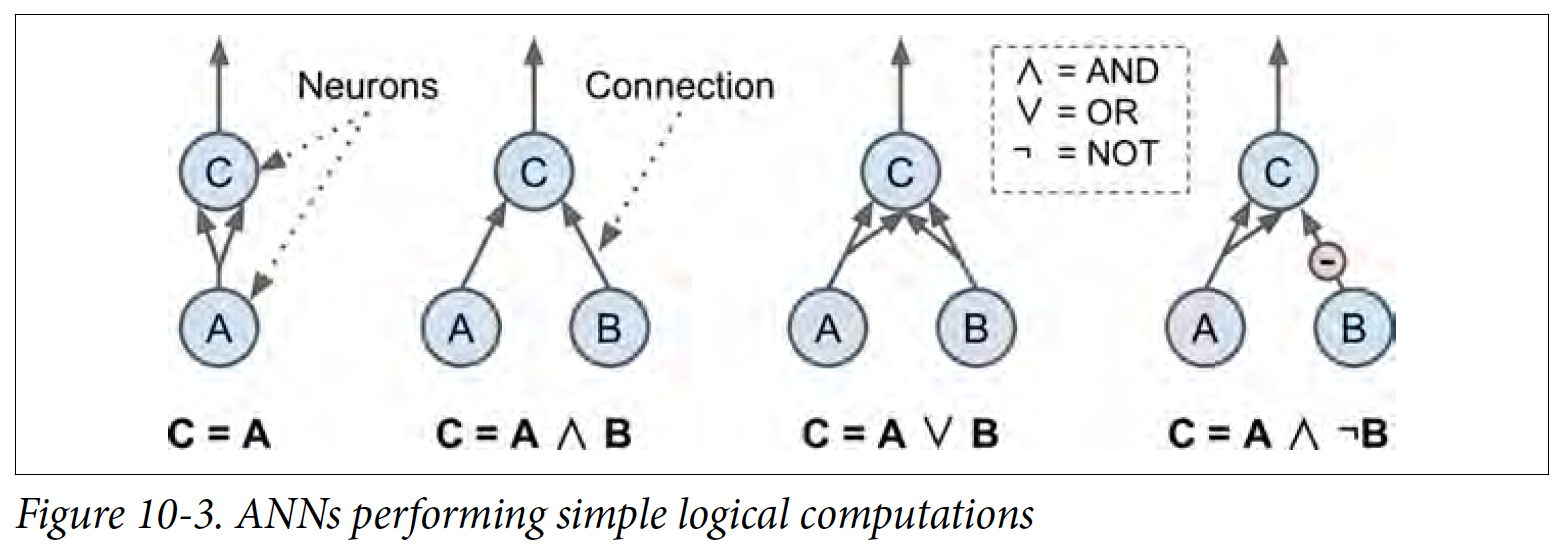
For 2 signals (in this case A and B), you can see with diagram how signals can lead up to stimulate the other neuron. In the textbook, it also leaves a question at the end : How would A XOR B look like?

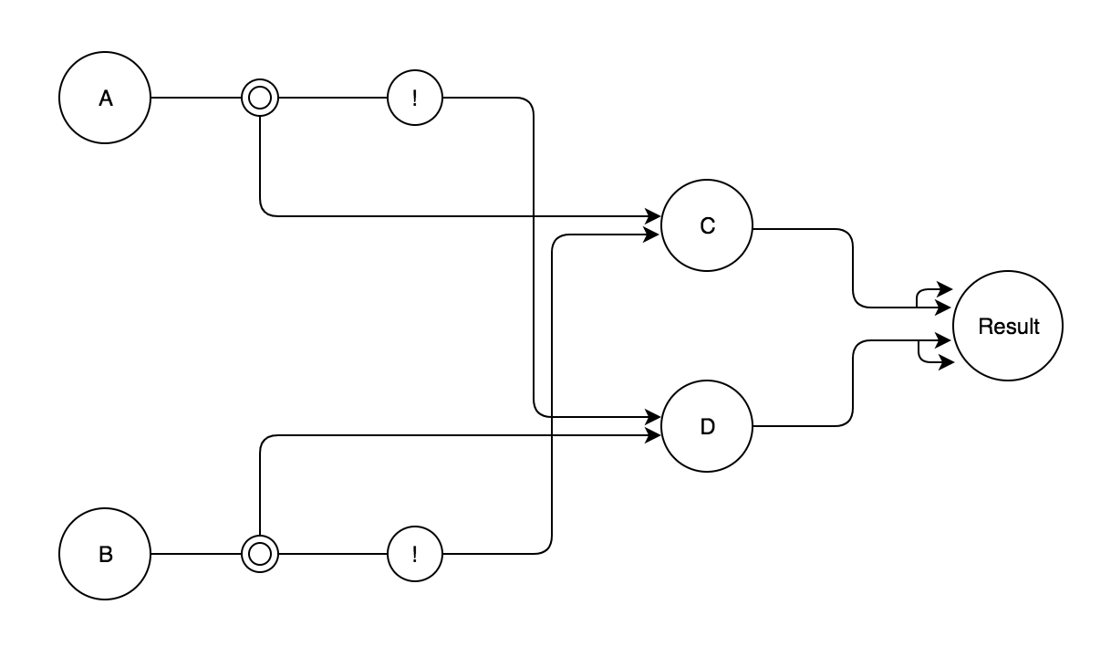
It didn’t really say if there could be intermediate nodes to get the inputs, so for the sake of a better looking graph, I’m going to assume there can be intermediate nodes to save a computed value. Here is my diagram.
Elaboration on Neural Network Optimization
Time to get our hands dirty with a bit of mathematical concepts! I’m going to leave out some maths out (i.e. chain rules and multiple differentiation) However, you do need to understand what taking a derivate of a certain function means.
Here is the first step
- Let there be n number of signals.
- x is when will either be 0 or 1 (it fires or doesn’t fire signals)
- w is weight
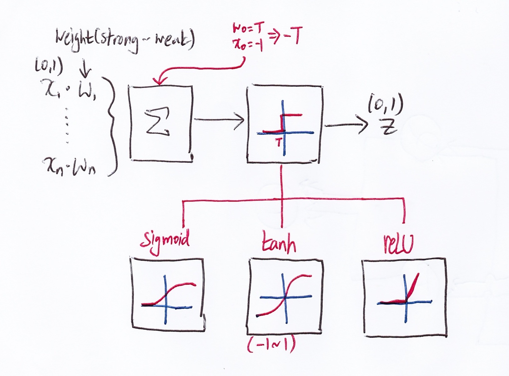
Note there is an -T input with the signal inputs. This is done for mathematical convenience (translating the T to origin). The figure below shows the translation.
![]()
Then there is 3 popular activation functions. Before I elaborate on those functions, a good question is, why do we need to transform a stepwise function (original) into another function? Later on when we try to find the maximum/minimum (depending on how you look at it), we’d have to use a optimization concept called gradient ascent/descent. The optimization that isn’t intractable can be only applied to continuous function (you have to take certain derivatives, but with stepwise, due to abrupt changes in the graph, derivatives falls apart). Thus, the stepwise function has to be transformed into a continuous function.
- sigmoid : this one is intuitive and is done quite a lot in the field of data analysis (i.e. if you have a questionnaire that has yes/no results, then normally a sigmoid is done on the data). However, this usually needs more computation and usually gives mediocre results compared to other activation function.
- tanh (Hyperbolic Tangent Function) : it’s pretty similar to sigmoid, but it helps speed up convergence due to stronger gradient caused by the larger range of the function.
- ReLU (Rectified Linear Unit) : there is a slight problem near origin due to abrupt change (i.e. it has mathematical problems when differentiated). However, due to it’s shape, it is faster to compute and reduces some issues with gradient ascent/descent. This function is the most popular currently
Now it’s time to move on the how this turns into a gradient ascent/descent problem. First we have an output z that can be compared to the desired (actual) result to measure performance, so that math goes like this.
![]()
Just incase the reader is not familiar why the values are in vector… since the desired and output have multiple values, it’s possible to think of them as a 1xN dimension matrix (where N = number of values), which is basically a vector.
If two vectors are just subtracted, it’s not very convenient for math (it’s a V shaped that can cause problems when differentiated), so the the whole performance is squared. Additionally, - is multiplied so that we can do gradient ascent (usually climbing is the norm). Of course there is no problem just using the positive value and use gradient descent. (for this blog I will keep using maximum + gradient ascent)
Now all we have to do is find the maximum. Now the problem can be taken on as shown below.
![]()
It’s explained above, but gradient ascent when done naively is exponential (intractable), so differentiation is used. When both in vertical and horizontal direction changes the most positively means that that is the optimal step to take.
Now with this we keep the weights adjusting so the neural network is modified to be closer and closer to the desired output!
Since overall theory of neural network is covered let’s move on to coding with Python… ‘^’

Applying Concepts into Python (with Tensorflow)
Perceptron is one of the simplest Artificial Neural Network (ANN) structure, so we’ll start at that. This one uses a threshold value (aka Linear Threshold Unit, meaning it does not use activation function to turn stepwise to continuous). In the textbook, it has a good visual example as shown below
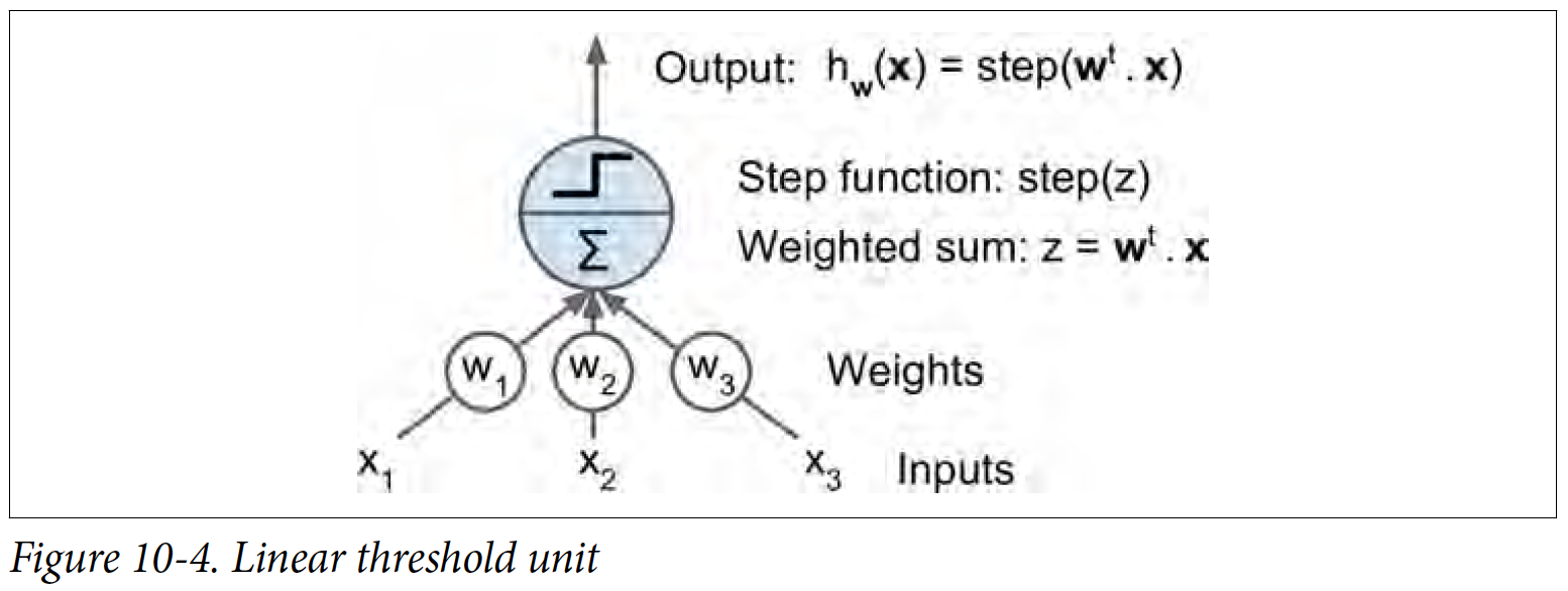
It works similar to one of the ML Algorithm, SVM (Support Vector Machine). There are different threshold ranges, but basically it classifies the inputs depending on if z is negative/positive.
I won’t be coding out the basic Perceptron codes on my blog, since I’d be just copy pasting exact same code as O’Reilly Machine Learning Book, so I strongly encourage you to visit the github created by the author that has all the codes and output.
Multi Layer Perceptron (MLP) is the next level for ANN structure. So there are inputs in the lower level, multiple perceptron in the middle level, and output on the upper level
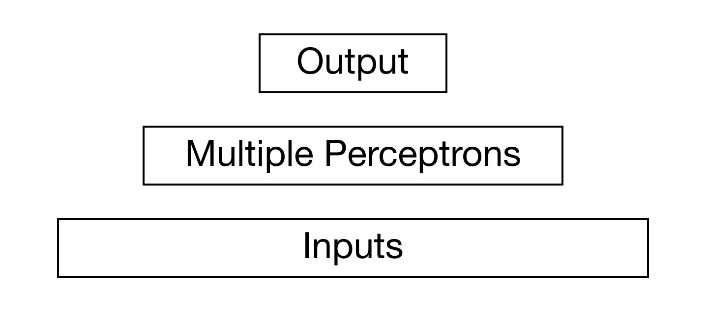
It’s possible to expand the MLP level into multiple level, which will result in a Deep Neural Network (DNN). As I mentioned previously, these multi-layer will look for neurons that contribute the most in the error and tweak their weights. We’ll now build a DNN in Tensorflow (also note most of the codes here are from O’Reilly Machine Learning Book). We will be building a DNN with 2 hidden layers (this is the most basic structure of a DNN).
Model
First we will load libraries and initialize variables
import tensorflow as tf
import numpy as np

input_dim = 28*28  # MNIST data is 28x28 pixels
hidden_1 = 300
hidden_2 = 100
output = 10 # there are 10 possible output -> 0,1,2,3,4,5,6,7,8,9

# tf.placeholder(dtype, shape, name)
# X = matrix instance * feature ; y = one entry instance
# shape None is used when training batch size is unknown
X = tf.placeholder(tf.float32, shape=(None, input_dim), name="X")
y = tf.placeholder(tf.int32, shape=(None), name="y")
Now the all the setup, it’s time to create define the model using Tensorflow. First starting with a user defined function of a neuron layer (note that there are built-in functions inside Tensorflow such as fully_connected, so you don’t actually have create a function. However, this post is for learning purposes ‘^’)
def neuron_layer(X, n_neurons, name, activation=None):
    with tf.name_scope(name):
        # creating weight matrix W
        n_inputs = int(X.get_shape()[1])
        std = 2 / np.sqrt(n_inputs) # this helps to converge much faster
        init = tf.truncated_normal((n_inputs, n_neurons),
                                    stddev=std) # truncated avoids large weights, so more efficient
        W = tf.Variable(init, name="kernel")
        # bias set to 0
        b = tf.Variable(tf.zeros([n_neurons]), name="bias")
        # Z (the output) = X (0 or 1) * W (weight) + b (bias)
        Z = tf.matmul(X, W) + b

        # activation default on ReLU
        if activation is not None:
            return activation(Z)
        else:
            return Z
Now that a neuron layer is defined, we move on to making hidden layer 1 -> hidden layer 2 -> output.
with tf.name_scope("dnn"):
    hidden1 = neuron_layer(X, hidden_1, name="hidden1", activation=tf.nn.relu)
    hidden2 = neuron_layer(hidden1, hidden_2, name="hidden2", activation=tf.nn.relu)
    logits = neuron_layer(hidden2, output, name="outputs") # note output = 10, so it will classify in 10 sections
Now that all the inputs have been turned into a value which have to be optimized and classified accordingly, now we need to start finding penalty values (as I mentioned before, in DNN, we take steps to reduce errors in multiple layers). In Machine Learning, this is related to loss/cost/error function (they are actually slightly different but in broad terms, they are synonymous).
if you are familiar with regression, you may think loss function as MSE
with tf.name_scope("loss"):
    xentropy = tf.nn.sparse_softmax_cross_entropy_with_logits(labels=y, logits=logits)
    loss = tf.reduce_mean(xentropy, name="loss")
Now that we have applied loss function, we have to add another step so that we minimize the errors. Since we are here to minimize instead of maximize, we’ll have to use a Gradient Descent Optimizer.
with tf.name_scope("train"):
    optimizer = tf.train.GradientDescentOptimizer(0.01) # learning rate
    training_op = optimizer.minimize(loss)
We have the penalty minimized, so now the model needs to choose which weights to tweak and keep. This will be the last step to build the model.
with tf.name_scope("eval"):
    correct = tf.nn.in_top_k(logits, y, 1)
    accuracy = tf.reduce_mean(tf.cast(correct, tf.float32))
Setting up before Execution
We ought to save our results to the local memory before executing and specify number of steps and batch.
init = tf.global_variables_initializer()
saver = tf.train.Saver()

n_epochs = 40 # this is the number of steps it will take
batch_size = 50

# getting MNIST data and splitting train and test
(X_train, y_train), (X_test, y_test) = tf.keras.datasets.mnist.load_data()
X_train = X_train.astype(np.float32).reshape(-1, 28*28) / 255.0
X_test = X_test.astype(np.float32).reshape(-1, 28*28) / 255.0
y_train = y_train.astype(np.int32)
y_test = y_test.astype(np.int32)

X_valid, X_train = X_train[:10000], X_train[10000:]
y_valid, y_train = y_train[:10000], y_train[10000:]
Execution
# shuffling (common practice)
def shuffle_batch(X, y, batch_size):
    rnd_idx = np.random.permutation(len(X))
    n_batches = len(X) // batch_size
    for batch_idx in np.array_split(rnd_idx, n_batches):
        X_batch, y_batch = X[batch_idx], y[batch_idx]
        yield X_batch, y_batch

with tf.Session() as sess:
    init.run()
    for epoch in range(n_epochs):
        for X_batch, y_batch in shuffle_batch(X_train, y_train, batch_size):
            sess.run(training_op, feed_dict={X: X_batch, y: y_batch})
        acc_batch = accuracy.eval(feed_dict={X: X_batch, y: y_batch})
        acc_val = accuracy.eval(feed_dict={X: X_valid, y: y_valid})
        print(epoch, "Batch accuracy:", acc_batch, "Val accuracy:", acc_val)
    save_path = saver.save(sess, "./my_model_final.ckpt")

# to look at the accuracy (saves accuracy into accuracy_val)
with tf.Session() as sess:
    saver.restore(sess, "./my_model_final.ckpt")
    accuracy_val = accuracy.eval(feed_dict={X: X_test, y: y_test})
Comments