Two-Level CNN for Lung Cancer Histology Classification

Abstract

This project classifies lung cancer histology images into 4 categories — Normal Cell (NORM), Small Cell (SCLC), Squamous Cell (SC), and Adenocarcinoma (ADC) — using a Convolutional Neural Network (CNN).

Traditional CNN image classification uses a one-level CNN where the whole image is processed in one pass. In this project, to reduce computational cost and push the network to capture more intricate details, a two-level CNN is used: Level 1 — Patch and Level 2 — Image.

Average accuracy on the validation set was 93% for Level 1 (Patch) and 97% for Level 2 (Image). On a held-out test set, the model classified 98.5% of images into the correct category.

Specifications

Images — 1,600 images per category (6,400 total), each 2,560 × 2,560 pixels. These images were extracted based on the doctor’s annotations on multiple whole-slide images.

Hardware

• OS — Windows 10
• RAM — 32GB
• CPU — 3.7GHz Intel Xeon E5-1630
• GPU — 2 × Nvidia GeForce GTX 1080 Ti (11GB)

Software

• Python 3.6.7
• PyTorch v0.3.0
• CUDA 9.0 Base
• cuDNN 7.4.2

Basic Visual Features

Four classes: Normal Cell (NORM), Small Cell (SCLC), Squamous Cell (SC), and Adenocarcinoma (ADC).

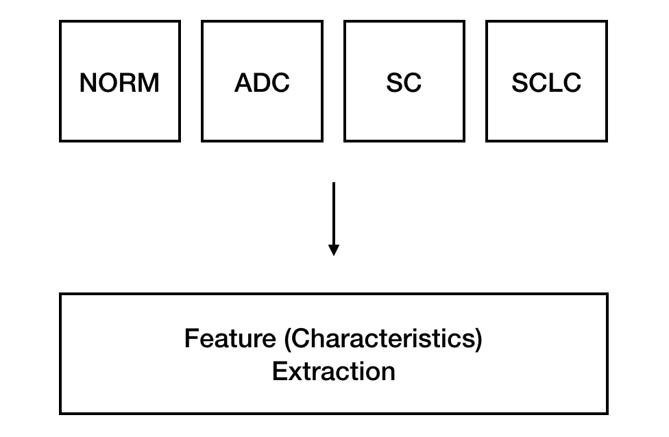The four target classes

The histology images below were handpicked to clearly show distinctive features for each category.

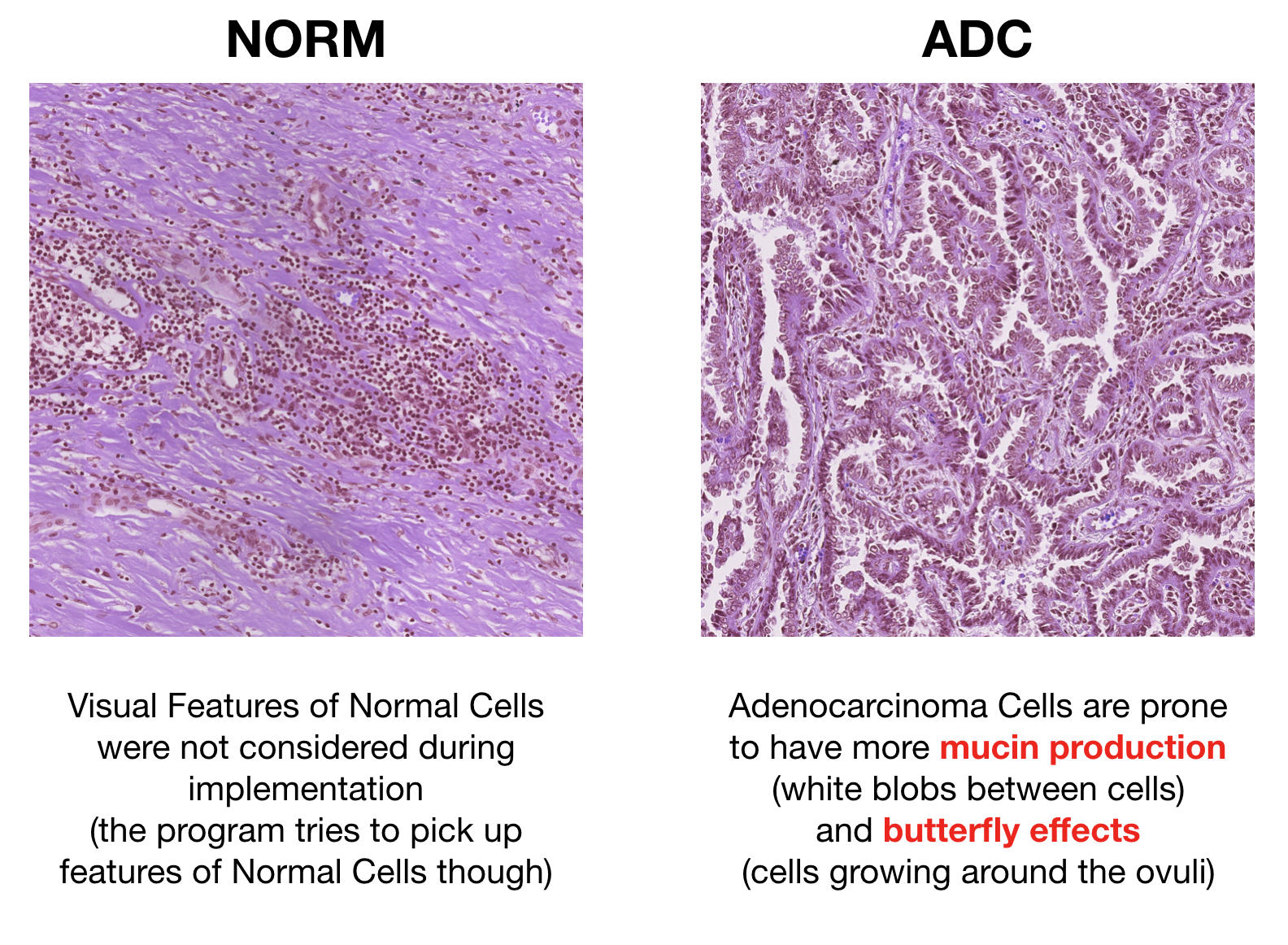NORM vs ADC — distinctive features

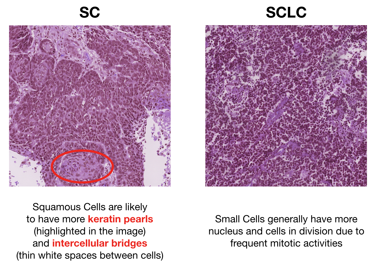SC vs SCLC — distinctive features

Program Structure

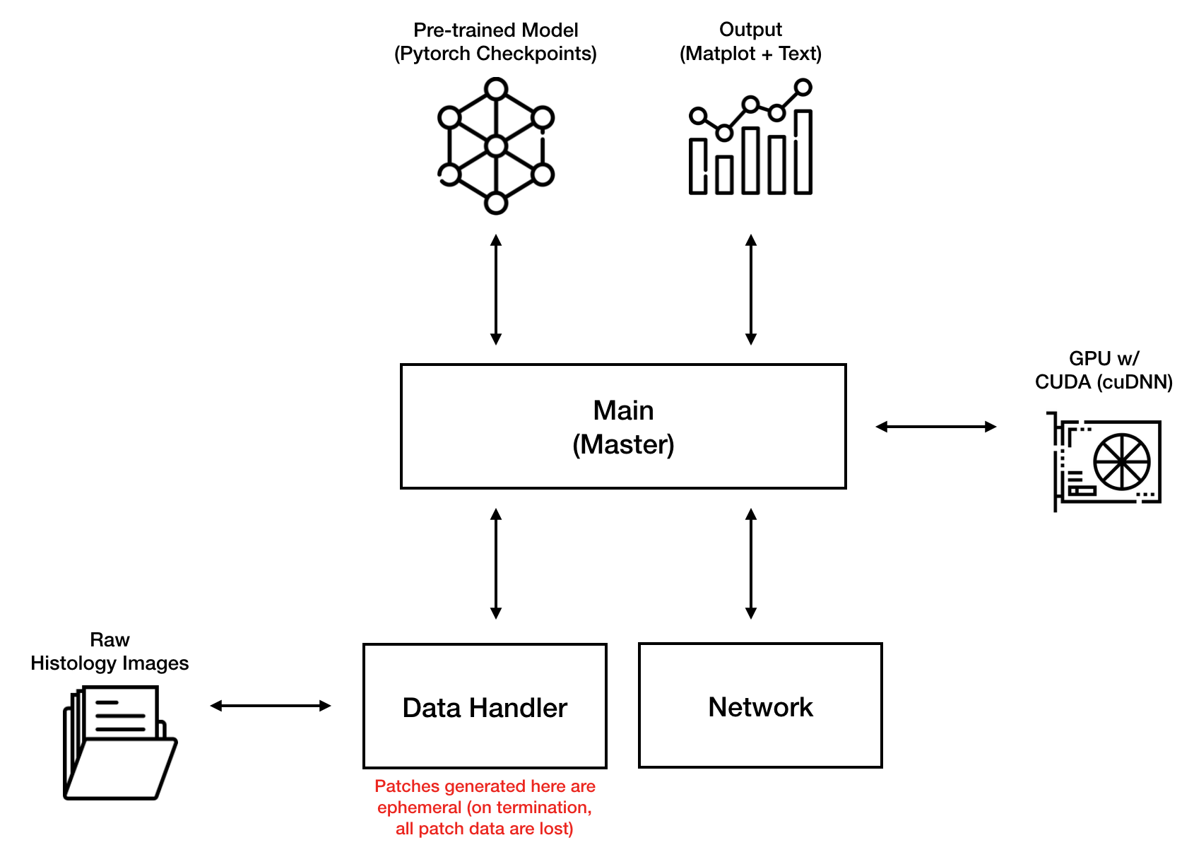End-to-end program architecture

Network Structure

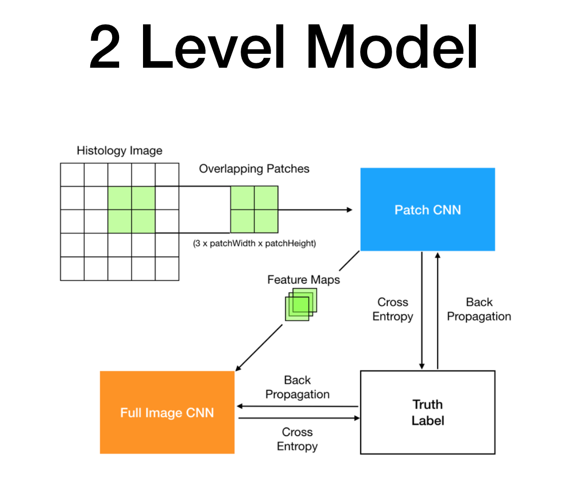Two-level network: patches → patch-level CNN → image-level CNN

Level 1 — Patch

Patch Extraction

Patches need to be sized appropriately for the network to pick up distinct per-class patterns, and the stride needs to be small enough to avoid losing spatial information between patches. Finding the optimal values via trial and error wasn’t realistic — a single full-scale training run would take weeks of compute. The patch size and stride were instead set based on prior CNN research on similar histology datasets.

• Patch Size — 512 pixels
• Stride — 256 pixels

For a 2,560 × 2,560 image, that gives (2560 − 512) / 256 + 1 = 9 patches per row × 9 per column = 81 patches per image. The patch network therefore sees roughly 388k training patches (4,800 training images × 81), not 4,800 — a much larger effective dataset.

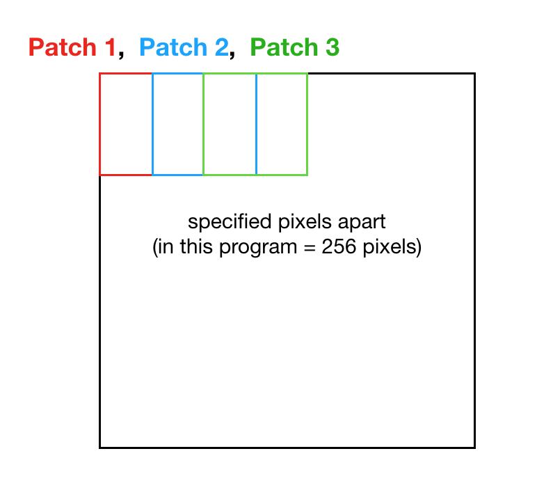Patch tiling with overlap (stride < patch size)

class ExtractPatches:
    def __init__(self, image, patchSize, stride):
        self.image = image
        self.patchSize = patchSize
        self.stride = stride

    def extract_single_patches(self, patch):
        croppedPatches = self.image.crop((patch[0] * self.stride, patch[1] * self.stride,
                                          patch[0] * self.stride + self.patchSize,
                                          patch[1] * self.stride + self.patchSize))

        return croppedPatches

    def no_of_patches(self):
        xNoOfPatches, yNoOfPatches = (int((self.image.width - self.patchSize) / self.stride + 1),
                                      int((self.image.height - self.patchSize) / self.stride + 1))

        return xNoOfPatches, yNoOfPatches

    def extract_all_patches(self):
        xNoOfPatches, yNoOfPatches = self.no_of_patches()

        allPatches = list()
        for y in range(yNoOfPatches):
            for x in range(xNoOfPatches):
                allPatches.append(self.extract_single_patches((x,y)))

        return allPatches

Patch Neural Network Architecture

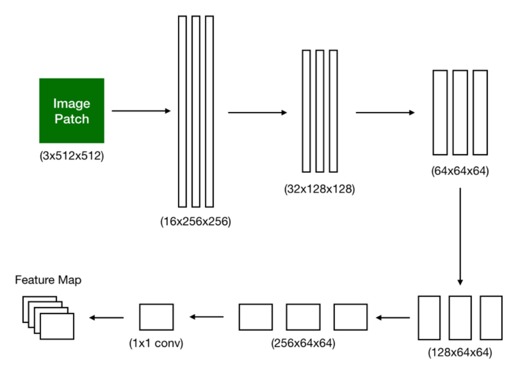Level 1: patch-level CNN architecture

BatchNorm2d is applied throughout the feature-extraction pipeline to stabilize training, with a mild regularization side-effect. Spatial dimensions are progressively shrunk via 2×2 stride-2 convs — the more common choice would be max-pooling, but here the learnable conv outperformed it on a held-out subset (presumably because it adds parameters max-pool doesn’t have).

The model is saved as a PyTorch checkpoint file after each epoch.

class PatchLevelNetwork(BaseNetwork):
    def __init__(self):
        super(PatchLevelNetwork, self).__init__('p_')

        self.features = nn.Sequential(
            nn.Conv2d(in_channels=3, out_channels=16, kernel_size=3, stride=1, padding=1),
            nn.BatchNorm2d(16),
            nn.ReLU(),
            nn.Conv2d(in_channels=16, out_channels=16, kernel_size=3, stride=1, padding=1),
            nn.BatchNorm2d(16),
            nn.ReLU(),
            nn.Conv2d(in_channels=16, out_channels=16, kernel_size=2, stride=2),
            nn.BatchNorm2d(16),
            nn.ReLU(),

            # middle blocks omitted — refer to the architecture diagram above
            # for the full layer sequence (channels grow toward 256;
            # 3 total 2×2 stride-2 downsamples take 512 → 64 spatial dim)

            nn.Conv2d(in_channels=128, out_channels=256, kernel_size=3, stride=1, padding=1),
            nn.BatchNorm2d(256),
            nn.ReLU(),
            nn.Conv2d(in_channels=256, out_channels=256, kernel_size=3, stride=1, padding=1),
            nn.BatchNorm2d(256),
            nn.ReLU(),
            nn.Conv2d(in_channels=256, out_channels=256, kernel_size=2, stride=2),
            nn.BatchNorm2d(256),
            nn.ReLU(),

            nn.Conv2d(in_channels=256, out_channels=1, kernel_size=1, stride=1),
        )

        self.classifier = nn.Sequential(
            nn.Linear(1 * 64 * 64, 4),
        )

        self.init_weight()

    def forward(self, x):
        x = self.features(x)
        x = x.view(x.size(0), -1)
        x = self.classifier(x)
        x = F.log_softmax(x, dim=1)
        return x

Level 2 — Image

Image Neural Network Architecture

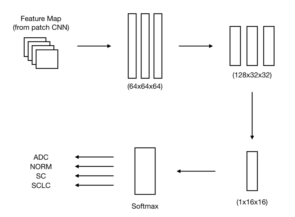Level 2: image-level CNN architecture (consumes Level 1 patch feature maps)

The full architecture code isn’t included because it’s largely the same as the patch network. The classifier differs — it adds dropout between every linear block to further reduce overfitting:

self.classifier = nn.Sequential(
    nn.Linear(1 * 16 * 16, 128),
    nn.ReLU(),
    nn.Dropout(0.5),

    nn.Linear(128, 128),
    nn.ReLU(),
    nn.Dropout(0.5),

    nn.Linear(128, 64),
    nn.ReLU(),
    nn.Dropout(0.5),

    nn.Linear(64, 4),
)

Results

Training & Validation Set

A total of 1,200 training images and 300 validation images per class (6,000 images total). Each epoch took about a day; the results below are from 20 epochs of training with the Adam optimizer.

• Learning rate — 0.001
• Beta1 — 0.9
• Beta2 — 0.999
• Log interval — 50 (log training loss every 50 batches)
• Epochs — 20

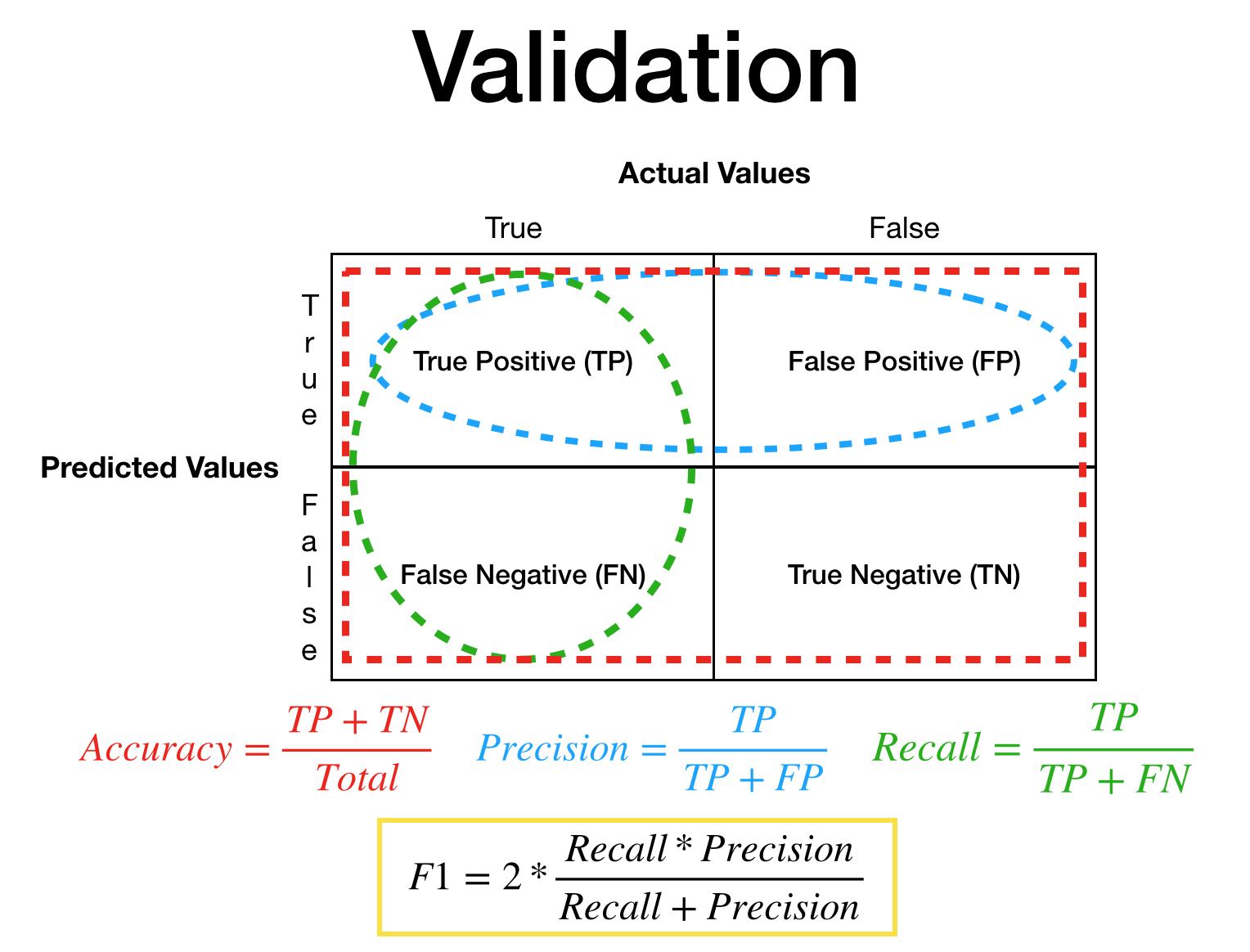Legend — what each value in the result plots represents

Per-level results

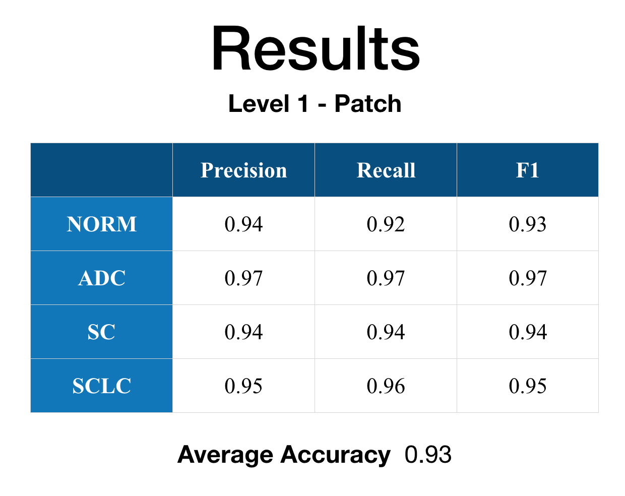Level 1 — patch-level training & validation curves

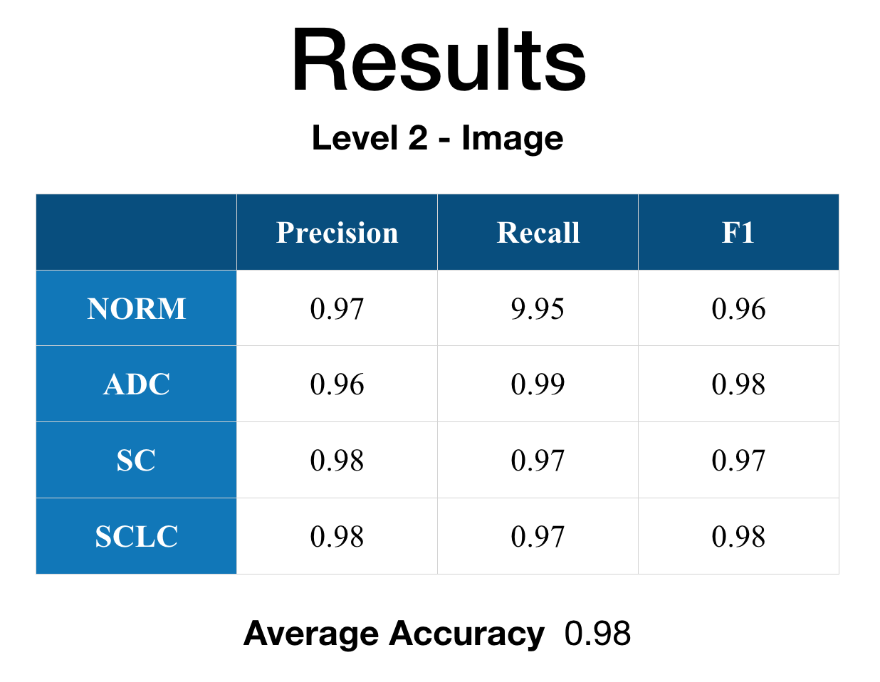Level 2 — image-level training & validation curves

ROC (Receiver Operating Characteristic)

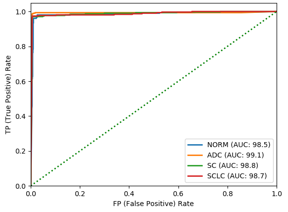ROC curve across the four classes

Looking through the results, some of the patches (not the whole images) contain significant white space with little cellular content, which drags down patch-level accuracy. Accuracy improves once the patch-level feature maps are fed into the image-level network, which can pool weak signals across many patches.

Test Set

A total of 100 unseen histology images per class (400 total) were held out from training.

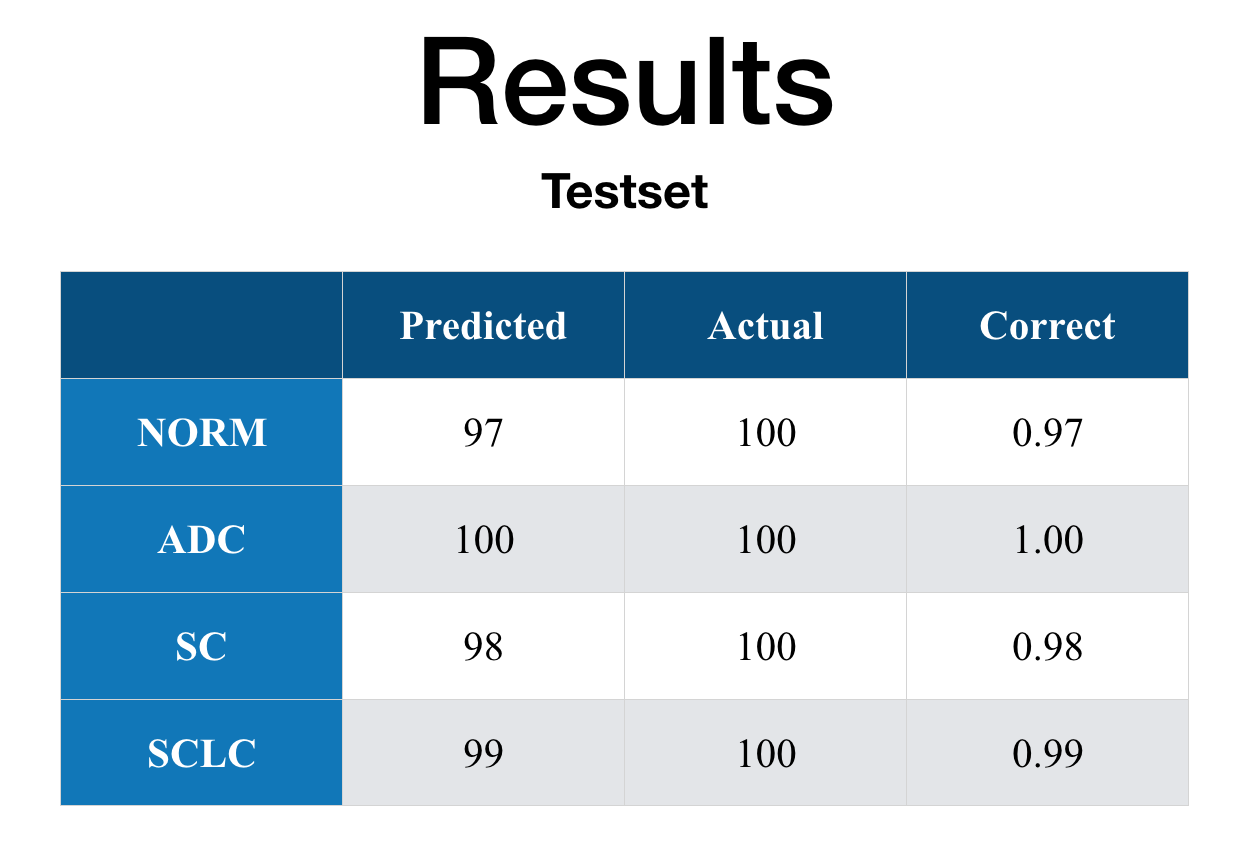Test set results — 98.5% classification accuracy